LSTMs for Human Activity Recognition
Human Activity Recognition (HAR) using smartphones dataset and an LSTM RNN. Classifying the type of movement amongst six categories:
- WALKING,
- WALKING_UPSTAIRS,
- WALKING_DOWNSTAIRS,
- SITTING,
- STANDING,
- LAYING.
Compared to a classical approach, using a Recurrent Neural Networks (RNN) with Long Short-Term Memory cells (LSTMs) require no or almost no feature engineering. Data can be fed directly into the neural network who acts like a black box, modeling the problem correctly. Other research on the activity recognition dataset can use a big amount of feature engineering, which is rather a signal processing approach combined with classical data science techniques. The approach here is rather very simple in terms of how much was the data preprocessed.
Let's use Google's neat Deep Learning library, TensorFlow, demonstrating the usage of an LSTM, a type of Artificial Neural Network that can process sequential data / time series.
Video dataset overview
Follow this link to see a video of the 6 activities recorded in the experiment with one of the participants:
[Watch video]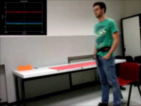
Details about the input data
I will be using an LSTM on the data to learn (as a cellphone attached on the waist) to recognise the type of activity that the user is doing. The dataset's description goes like this:
The sensor signals (accelerometer and gyroscope) were pre-processed by applying noise filters and then sampled in fixed-width sliding windows of 2.56 sec and 50% overlap (128 readings/window). The sensor acceleration signal, which has gravitational and body motion components, was separated using a Butterworth low-pass filter into body acceleration and gravity. The gravitational force is assumed to have only low frequency components, therefore a filter with 0.3 Hz cutoff frequency was used.
That said, I will use the almost raw data: only the gravity effect has been filtered out of the accelerometer as a preprocessing step for another 3D feature as an input to help learning. If you'd ever want to extract the gravity by yourself, you could fork my code on using a Butterworth Low-Pass Filter (LPF) in Python and edit it to have the right cutoff frequency of 0.3 Hz which is a good frequency for activity recognition from body sensors.
What is an RNN?
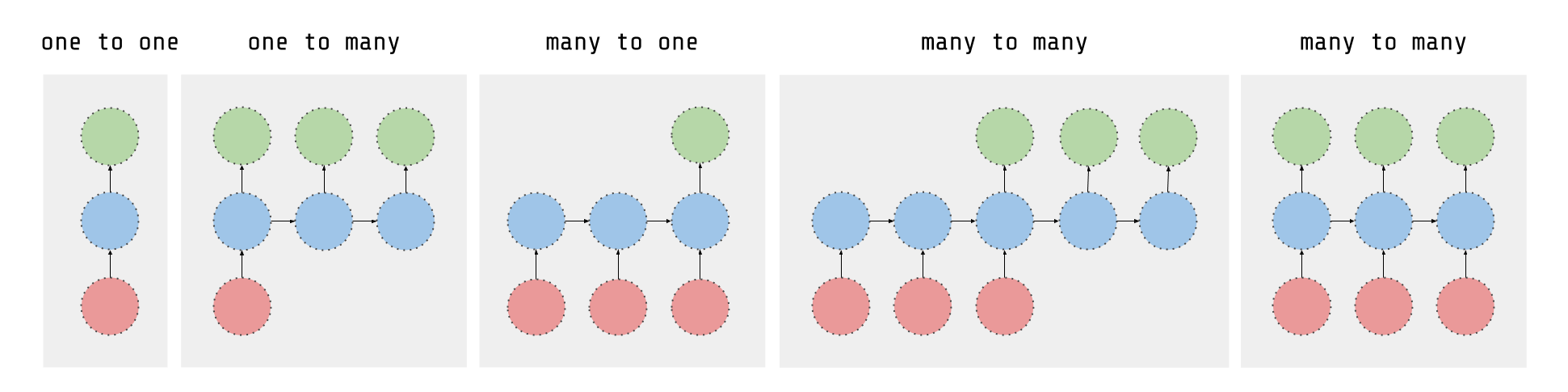
As explained in this article, an RNN takes many input vectors to process them and output other vectors. It can be roughly pictured like in the image below, imagining each rectangle has a vectorial depth and other special hidden quirks in the image below. In our case, the "many to one" architecture is used: we accept time series of feature vectors (one vector per time step) to convert them to a probability vector at the output for classification. Note that a "one to one" architecture would be a standard feedforward neural network.
What is an LSTM?
An LSTM is an improved RNN. It is more complex, but easier to train, avoiding what is called the vanishing gradient problem. I recommend this course for you to learn more on LSTMs.
Results
Scroll on! Nice visuals awaits.
# All Includes

import numpy as np
import matplotlib
import matplotlib.pyplot as plt
import tensorflow as tf  # Version 1.0.0 (some previous versions are used in past commits)
from sklearn import metrics

import os
# Useful Constants

# Those are separate normalised input features for the neural network
INPUT_SIGNAL_TYPES = [
    "body_acc_x_",
    "body_acc_y_",
    "body_acc_z_",
    "body_gyro_x_",
    "body_gyro_y_",
    "body_gyro_z_",
    "total_acc_x_",
    "total_acc_y_",
    "total_acc_z_"
]

# Output classes to learn how to classify
LABELS = [
    "WALKING",
    "WALKING_UPSTAIRS",
    "WALKING_DOWNSTAIRS",
    "SITTING",
    "STANDING",
    "LAYING"
]
Let's start by downloading the data:
# Note: Linux bash commands start with a "!" inside those "ipython notebook" cells

DATA_PATH = "data/"

!pwd && ls
os.chdir(DATA_PATH)
!pwd && ls

!python download_dataset.py

!pwd && ls
os.chdir("..")
!pwd && ls

DATASET_PATH = DATA_PATH + "UCI HAR Dataset/"
print("\n" + "Dataset is now located at: " + DATASET_PATH)
/home/ubuntu/pynb/LSTM-Human-Activity-Recognition
data	 LSTM_files  LSTM_OLD.ipynb  README.md
LICENSE  LSTM.ipynb  lstm.py	     screenlog.0
/home/ubuntu/pynb/LSTM-Human-Activity-Recognition/data
download_dataset.py  source.txt

Downloading...
--2017-05-24 01:49:53--  https://archive.ics.uci.edu/ml/machine-learning-databases/00240/UCI%20HAR%20Dataset.zip
Resolving archive.ics.uci.edu (archive.ics.uci.edu)... 128.195.10.249
Connecting to archive.ics.uci.edu (archive.ics.uci.edu)|128.195.10.249|:443... connected.
HTTP request sent, awaiting response... 200 OK
Length: 60999314 (58M) [application/zip]
Saving to: ‘UCI HAR Dataset.zip’

100%[======================================>] 60,999,314  1.69MB/s   in 38s

2017-05-24 01:50:31 (1.55 MB/s) - ‘UCI HAR Dataset.zip’ saved [60999314/60999314]

Downloading done.

Extracting...
Extracting successfully done to /home/ubuntu/pynb/LSTM-Human-Activity-Recognition/data/UCI HAR Dataset.
/home/ubuntu/pynb/LSTM-Human-Activity-Recognition/data
download_dataset.py  __MACOSX  source.txt  UCI HAR Dataset  UCI HAR Dataset.zip
/home/ubuntu/pynb/LSTM-Human-Activity-Recognition
data	 LSTM_files  LSTM_OLD.ipynb  README.md
LICENSE  LSTM.ipynb  lstm.py	     screenlog.0

Dataset is now located at: data/UCI HAR Dataset/
Preparing dataset:
TRAIN = "train/"
TEST = "test/"


# Load "X" (the neural network's training and testing inputs)

def load_X(X_signals_paths):
    X_signals = []

    for signal_type_path in X_signals_paths:
        file = open(signal_type_path, 'r')
        # Read dataset from disk, dealing with text files' syntax
        X_signals.append(
            [np.array(serie, dtype=np.float32) for serie in [
                row.replace('  ', ' ').strip().split(' ') for row in file
            ]]
        )
        file.close()

    return np.transpose(np.array(X_signals), (1, 2, 0))

X_train_signals_paths = [
    DATASET_PATH + TRAIN + "Inertial Signals/" + signal + "train.txt" for signal in INPUT_SIGNAL_TYPES
]
X_test_signals_paths = [
    DATASET_PATH + TEST + "Inertial Signals/" + signal + "test.txt" for signal in INPUT_SIGNAL_TYPES
]

X_train = load_X(X_train_signals_paths)
X_test = load_X(X_test_signals_paths)


# Load "y" (the neural network's training and testing outputs)

def load_y(y_path):
    file = open(y_path, 'r')
    # Read dataset from disk, dealing with text file's syntax
    y_ = np.array(
        [elem for elem in [
            row.replace('  ', ' ').strip().split(' ') for row in file
        ]],
        dtype=np.int32
    )
    file.close()

    # Substract 1 to each output class for friendly 0-based indexing
    return y_ - 1

y_train_path = DATASET_PATH + TRAIN + "y_train.txt"
y_test_path = DATASET_PATH + TEST + "y_test.txt"

y_train = load_y(y_train_path)
y_test = load_y(y_test_path)
Additionnal Parameters:
Here are some core parameter definitions for the training.
For example, the whole neural network's structure could be summarised by enumerating those parameters and the fact that two LSTM are used one on top of another (stacked) output-to-input as hidden layers through time steps.
# Input Data

training_data_count = len(X_train)  # 7352 training series (with 50% overlap between each serie)
test_data_count = len(X_test)  # 2947 testing series
n_steps = len(X_train[0])  # 128 timesteps per series
n_input = len(X_train[0][0])  # 9 input parameters per timestep


# LSTM Neural Network's internal structure

n_hidden = 32 # Hidden layer num of features
n_classes = 6 # Total classes (should go up, or should go down)


# Training

learning_rate = 0.0025
lambda_loss_amount = 0.0015
training_iters = training_data_count * 300  # Loop 300 times on the dataset
batch_size = 1500
display_iter = 30000  # To show test set accuracy during training


# Some debugging info

print("Some useful info to get an insight on dataset's shape and normalisation:")
print("(X shape, y shape, every X's mean, every X's standard deviation)")
print(X_test.shape, y_test.shape, np.mean(X_test), np.std(X_test))
print("The dataset is therefore properly normalised, as expected, but not yet one-hot encoded.")
Some useful info to get an insight on dataset's shape and normalisation:
(X shape, y shape, every X's mean, every X's standard deviation)
(2947, 128, 9) (2947, 1) 0.0991399 0.395671
The dataset is therefore properly normalised, as expected, but not yet one-hot encoded.
Utility functions for training:
def LSTM_RNN(_X, _weights, _biases):
    # Function returns a tensorflow LSTM (RNN) artificial neural network from given parameters.
    # Moreover, two LSTM cells are stacked which adds deepness to the neural network.
    # Note, some code of this notebook is inspired from an slightly different
    # RNN architecture used on another dataset, some of the credits goes to
    # "aymericdamien" under the MIT license.

    # (NOTE: This step could be greatly optimised by shaping the dataset once
    # input shape: (batch_size, n_steps, n_input)
    _X = tf.transpose(_X, [1, 0, 2])  # permute n_steps and batch_size
    # Reshape to prepare input to hidden activation
    _X = tf.reshape(_X, [-1, n_input])
    # new shape: (n_steps*batch_size, n_input)

    # ReLU activation, thanks to Yu Zhao for adding this improvement here:
    _X = tf.nn.relu(tf.matmul(_X, _weights['hidden']) + _biases['hidden'])
    # Split data because rnn cell needs a list of inputs for the RNN inner loop
    _X = tf.split(_X, n_steps, 0)
    # new shape: n_steps * (batch_size, n_hidden)

    # Define two stacked LSTM cells (two recurrent layers deep) with tensorflow
    lstm_cell_1 = tf.contrib.rnn.BasicLSTMCell(n_hidden, forget_bias=1.0, state_is_tuple=True)
    lstm_cell_2 = tf.contrib.rnn.BasicLSTMCell(n_hidden, forget_bias=1.0, state_is_tuple=True)
    lstm_cells = tf.contrib.rnn.MultiRNNCell([lstm_cell_1, lstm_cell_2], state_is_tuple=True)
    # Get LSTM cell output
    outputs, states = tf.contrib.rnn.static_rnn(lstm_cells, _X, dtype=tf.float32)

    # Get last time step's output feature for a "many-to-one" style classifier,
    # as in the image describing RNNs at the top of this page
    lstm_last_output = outputs[-1]

    # Linear activation
    return tf.matmul(lstm_last_output, _weights['out']) + _biases['out']


def extract_batch_size(_train, step, batch_size):
    # Function to fetch a "batch_size" amount of data from "(X|y)_train" data.

    shape = list(_train.shape)
    shape[0] = batch_size
    batch_s = np.empty(shape)

    for i in range(batch_size):
        # Loop index
        index = ((step-1)*batch_size + i) % len(_train)
        batch_s[i] = _train[index]

    return batch_s


def one_hot(y_, n_classes=n_classes):
    # Function to encode neural one-hot output labels from number indexes
    # e.g.:
    # one_hot(y_=[[5], [0], [3]], n_classes=6):
    #     return [[0, 0, 0, 0, 0, 1], [1, 0, 0, 0, 0, 0], [0, 0, 0, 1, 0, 0]]

    y_ = y_.reshape(len(y_))
    return np.eye(n_classes)[np.array(y_, dtype=np.int32)]  # Returns FLOATS
Let's get serious and build the neural network:
# Graph input/output
x = tf.placeholder(tf.float32, [None, n_steps, n_input])
y = tf.placeholder(tf.float32, [None, n_classes])

# Graph weights
weights = {
    'hidden': tf.Variable(tf.random_normal([n_input, n_hidden])), # Hidden layer weights
    'out': tf.Variable(tf.random_normal([n_hidden, n_classes], mean=1.0))
}
biases = {
    'hidden': tf.Variable(tf.random_normal([n_hidden])),
    'out': tf.Variable(tf.random_normal([n_classes]))
}

pred = LSTM_RNN(x, weights, biases)

# Loss, optimizer and evaluation
l2 = lambda_loss_amount * sum(
    tf.nn.l2_loss(tf_var) for tf_var in tf.trainable_variables()
) # L2 loss prevents this overkill neural network to overfit the data
cost = tf.reduce_mean(tf.nn.softmax_cross_entropy_with_logits(labels=y, logits=pred)) + l2 # Softmax loss
optimizer = tf.train.AdamOptimizer(learning_rate=learning_rate).minimize(cost) # Adam Optimizer

correct_pred = tf.equal(tf.argmax(pred,1), tf.argmax(y,1))
accuracy = tf.reduce_mean(tf.cast(correct_pred, tf.float32))
Hooray, now train the neural network:
# To keep track of training's performance
test_losses = []
test_accuracies = []
train_losses = []
train_accuracies = []

# Launch the graph
sess = tf.InteractiveSession(config=tf.ConfigProto(log_device_placement=True))
init = tf.global_variables_initializer()
sess.run(init)

# Perform Training steps with "batch_size" amount of example data at each loop
step = 1
while step * batch_size <= training_iters:
    batch_xs =         extract_batch_size(X_train, step, batch_size)
    batch_ys = one_hot(extract_batch_size(y_train, step, batch_size))

    # Fit training using batch data
    _, loss, acc = sess.run(
        [optimizer, cost, accuracy],
        feed_dict={
            x: batch_xs,
            y: batch_ys
        }
    )
    train_losses.append(loss)
    train_accuracies.append(acc)

    # Evaluate network only at some steps for faster training:
    if (step*batch_size % display_iter == 0) or (step == 1) or (step * batch_size > training_iters):

        # To not spam console, show training accuracy/loss in this "if"
        print("Training iter #" + str(step*batch_size) + \
              ":   Batch Loss = " + "{:.6f}".format(loss) + \
              ", Accuracy = {}".format(acc))

        # Evaluation on the test set (no learning made here - just evaluation for diagnosis)
        loss, acc = sess.run(
            [cost, accuracy],
            feed_dict={
                x: X_test,
                y: one_hot(y_test)
            }
        )
        test_losses.append(loss)
        test_accuracies.append(acc)
        print("PERFORMANCE ON TEST SET: " + \
              "Batch Loss = {}".format(loss) + \
              ", Accuracy = {}".format(acc))

    step += 1

print("Optimization Finished!")

# Accuracy for test data

one_hot_predictions, accuracy, final_loss = sess.run(
    [pred, accuracy, cost],
    feed_dict={
        x: X_test,
        y: one_hot(y_test)
    }
)

test_losses.append(final_loss)
test_accuracies.append(accuracy)

print("FINAL RESULT: " + \
      "Batch Loss = {}".format(final_loss) + \
      ", Accuracy = {}".format(accuracy))
WARNING:tensorflow:From <ipython-input-19-3339689e51f6>:9: initialize_all_variables (from tensorflow.python.ops.variables) is deprecated and will be removed after 2017-03-02.
Instructions for updating:
Use `tf.global_variables_initializer` instead.
Training iter #1500:   Batch Loss = 5.416760, Accuracy = 0.15266665816307068
PERFORMANCE ON TEST SET: Batch Loss = 4.880829811096191, Accuracy = 0.05632847175002098
Training iter #30000:   Batch Loss = 3.031930, Accuracy = 0.607333242893219
PERFORMANCE ON TEST SET: Batch Loss = 3.0515167713165283, Accuracy = 0.6067186594009399
Training iter #60000:   Batch Loss = 2.672764, Accuracy = 0.7386666536331177
PERFORMANCE ON TEST SET: Batch Loss = 2.780435085296631, Accuracy = 0.7027485370635986
Training iter #90000:   Batch Loss = 2.378301, Accuracy = 0.8366667032241821
PERFORMANCE ON TEST SET: Batch Loss = 2.6019773483276367, Accuracy = 0.7617915868759155
Training iter #120000:   Batch Loss = 2.127290, Accuracy = 0.9066667556762695
PERFORMANCE ON TEST SET: Batch Loss = 2.3625404834747314, Accuracy = 0.8116728663444519
Training iter #150000:   Batch Loss = 1.929805, Accuracy = 0.9380000233650208
PERFORMANCE ON TEST SET: Batch Loss = 2.306251049041748, Accuracy = 0.8276212215423584
Training iter #180000:   Batch Loss = 1.971904, Accuracy = 0.9153333902359009
PERFORMANCE ON TEST SET: Batch Loss = 2.0835530757904053, Accuracy = 0.8771631121635437
Training iter #210000:   Batch Loss = 1.860249, Accuracy = 0.8613333702087402
PERFORMANCE ON TEST SET: Batch Loss = 1.9994492530822754, Accuracy = 0.8788597583770752
Training iter #240000:   Batch Loss = 1.626292, Accuracy = 0.9380000233650208
PERFORMANCE ON TEST SET: Batch Loss = 1.879166603088379, Accuracy = 0.8944689035415649
Training iter #270000:   Batch Loss = 1.582758, Accuracy = 0.9386667013168335
PERFORMANCE ON TEST SET: Batch Loss = 2.0341007709503174, Accuracy = 0.8361043930053711
Training iter #300000:   Batch Loss = 1.620352, Accuracy = 0.9306666851043701
PERFORMANCE ON TEST SET: Batch Loss = 1.8185184001922607, Accuracy = 0.8639293313026428
Training iter #330000:   Batch Loss = 1.474394, Accuracy = 0.9693333506584167
PERFORMANCE ON TEST SET: Batch Loss = 1.7638503313064575, Accuracy = 0.8747878670692444
Training iter #360000:   Batch Loss = 1.406998, Accuracy = 0.9420000314712524
PERFORMANCE ON TEST SET: Batch Loss = 1.5946787595748901, Accuracy = 0.902273416519165
Training iter #390000:   Batch Loss = 1.362515, Accuracy = 0.940000057220459
PERFORMANCE ON TEST SET: Batch Loss = 1.5285792350769043, Accuracy = 0.9046487212181091
Training iter #420000:   Batch Loss = 1.252860, Accuracy = 0.9566667079925537
PERFORMANCE ON TEST SET: Batch Loss = 1.4635565280914307, Accuracy = 0.9107565879821777
Training iter #450000:   Batch Loss = 1.190078, Accuracy = 0.9553333520889282
...
PERFORMANCE ON TEST SET: Batch Loss = 0.42567864060401917, Accuracy = 0.9324736595153809
Training iter #2070000:   Batch Loss = 0.342763, Accuracy = 0.9326667189598083
PERFORMANCE ON TEST SET: Batch Loss = 0.4292983412742615, Accuracy = 0.9273836612701416
Training iter #2100000:   Batch Loss = 0.259442, Accuracy = 0.9873334169387817
PERFORMANCE ON TEST SET: Batch Loss = 0.44131210446357727, Accuracy = 0.9273836612701416
Training iter #2130000:   Batch Loss = 0.284630, Accuracy = 0.9593333601951599
PERFORMANCE ON TEST SET: Batch Loss = 0.46982717514038086, Accuracy = 0.9093992710113525
Training iter #2160000:   Batch Loss = 0.299012, Accuracy = 0.9686667323112488
PERFORMANCE ON TEST SET: Batch Loss = 0.48389002680778503, Accuracy = 0.9138105511665344
Training iter #2190000:   Batch Loss = 0.287106, Accuracy = 0.9700000286102295
PERFORMANCE ON TEST SET: Batch Loss = 0.4670214056968689, Accuracy = 0.9216151237487793
Optimization Finished!
FINAL RESULT: Batch Loss = 0.45611169934272766, Accuracy = 0.9165252447128296
Training is good, but having visual insight is even better:
Okay, let's plot this simply in the notebook for now.
# (Inline plots: )
%matplotlib inline

font = {
    'family' : 'Bitstream Vera Sans',
    'weight' : 'bold',
    'size'   : 18
}
matplotlib.rc('font', **font)

width = 12
height = 12
plt.figure(figsize=(width, height))

indep_train_axis = np.array(range(batch_size, (len(train_losses)+1)*batch_size, batch_size))
plt.plot(indep_train_axis, np.array(train_losses),     "b--", label="Train losses")
plt.plot(indep_train_axis, np.array(train_accuracies), "g--", label="Train accuracies")

indep_test_axis = np.append(
    np.array(range(batch_size, len(test_losses)*display_iter, display_iter)[:-1]),
    [training_iters]
)
plt.plot(indep_test_axis, np.array(test_losses),     "b-", label="Test losses")
plt.plot(indep_test_axis, np.array(test_accuracies), "g-", label="Test accuracies")

plt.title("Training session's progress over iterations")
plt.legend(loc='upper right', shadow=True)
plt.ylabel('Training Progress (Loss or Accuracy values)')
plt.xlabel('Training iteration')

plt.show()

And finally, the multi-class confusion matrix and metrics!
# Results

predictions = one_hot_predictions.argmax(1)

print("Testing Accuracy: {}%".format(100*accuracy))

print("")
print("Precision: {}%".format(100*metrics.precision_score(y_test, predictions, average="weighted")))
print("Recall: {}%".format(100*metrics.recall_score(y_test, predictions, average="weighted")))
print("f1_score: {}%".format(100*metrics.f1_score(y_test, predictions, average="weighted")))

print("")
print("Confusion Matrix:")
confusion_matrix = metrics.confusion_matrix(y_test, predictions)
print(confusion_matrix)
normalised_confusion_matrix = np.array(confusion_matrix, dtype=np.float32)/np.sum(confusion_matrix)*100

print("")
print("Confusion matrix (normalised to % of total test data):")
print(normalised_confusion_matrix)
print("Note: training and testing data is not equally distributed amongst classes, ")
print("so it is normal that more than a 6th of the data is correctly classifier in the last category.")

# Plot Results:
width = 12
height = 12
plt.figure(figsize=(width, height))
plt.imshow(
    normalised_confusion_matrix,
    interpolation='nearest',
    cmap=plt.cm.rainbow
)
plt.title("Confusion matrix \n(normalised to % of total test data)")
plt.colorbar()
tick_marks = np.arange(n_classes)
plt.xticks(tick_marks, LABELS, rotation=90)
plt.yticks(tick_marks, LABELS)
plt.tight_layout()
plt.ylabel('True label')
plt.xlabel('Predicted label')
plt.show()
Testing Accuracy: 91.65252447128296%

Precision: 91.76286479743305%
Recall: 91.65252799457076%
f1_score: 91.6437546304815%

Confusion Matrix:
[[466   2  26   0   2   0]
 [  5 441  25   0   0   0]
 [  1   0 419   0   0   0]
 [  1   1   0 396  87   6]
 [  2   1   0  87 442   0]
 [  0   0   0   0   0 537]]

Confusion matrix (normalised to % of total test data):
[[ 15.81269073   0.06786563   0.88225317   0.           0.06786563   0.        ]
 [  0.16966406  14.96437073   0.84832031   0.           0.           0.        ]
 [  0.03393281   0.          14.21784878   0.           0.           0.        ]
 [  0.03393281   0.03393281   0.          13.43739319   2.95215464
    0.20359688]
 [  0.06786563   0.03393281   0.           2.95215464  14.99830341   0.        ]
 [  0.           0.           0.           0.           0.          18.22192001]]
Note: training and testing data is not equally distributed amongst classes,
so it is normal that more than a 6th of the data is correctly classifier in the last category.

sess.close()
Conclusion
Outstandingly, the final accuracy is of 91%! And it can peak to values such as 93.25%, at some moments of luck during the training, depending on how the neural network's weights got initialized at the start of the training, randomly.
This means that the neural networks is almost always able to correctly identify the movement type! Remember, the phone is attached on the waist and each series to classify has just a 128 sample window of two internal sensors (a.k.a. 2.56 seconds at 50 FPS), so it amazes me how those predictions are extremely accurate given this small window of context and raw data. I've validated and re-validated that there is no important bug, and the community used and tried this code a lot. (Note: be sure to report something in the issue tab if you find bugs, otherwise Quora, StackOverflow, and other StackExchange sites are the places for asking questions.)
I specially did not expect such good results for guessing between the labels "SITTING" and "STANDING". Those are seemingly almost the same thing from the point of view of a device placed at waist level according to how the dataset was originally gathered. Thought, it is still possible to see a little cluster on the matrix between those classes, which drifts away just a bit from the identity. This is great.
It is also possible to see that there was a slight difficulty in doing the difference between "WALKING", "WALKING_UPSTAIRS" and "WALKING_DOWNSTAIRS". Obviously, those activities are quite similar in terms of movements.
I also tried my code without the gyroscope, using only the 3D accelerometer's 6 features (and not changing the training hyperparameters), and got an accuracy of 87%. In general, gyroscopes consumes more power than accelerometers, so it is preferable to turn them off.
Improvements
In another open-source repository of mine, the accuracy is pushed up to nearly 94% using a special deep LSTM architecture which combines the concepts of bidirectional RNNs, residual connections, and stacked cells. This architecture is also tested on another similar activity dataset. It resembles the nice architecture used in "Google’s Neural Machine Translation System: Bridging the Gap between Human and Machine Translation", without an attention mechanism, and with just the encoder part - as a "many to one" architecture instead of a "many to many" to be adapted to the Human Activity Recognition (HAR) problem. I also worked more on the problem and came up with the LARNN, however it's complicated for just a little gain. Thus the current, original activity recognition project is simply better to use for its simplicity. We've also coded a non-deep learning machine learning pipeline on the same datasets using classical featurization techniques and older machine learning algorithms.
If you want to learn more about deep learning, I have also built a list of the learning ressources for deep learning which have revealed to be the most useful to me here. You may also be interested in my online course on Deep Learning and Recurrent Neural Networks (DL&RNN).
I also have made even more improvements as seen just below with the few lines of code for easier usage and for reaching an even better score. Note this this is still an ongoing project, subscribe here to learn more.
More time series processing
Visit Neuraxio's Time Series Solution product page for more information.
References
The dataset can be found on the UCI Machine Learning Repository:
Davide Anguita, Alessandro Ghio, Luca Oneto, Xavier Parra and Jorge L. Reyes-Ortiz. A Public Domain Dataset for Human Activity Recognition Using Smartphones. 21th European Symposium on Artificial Neural Networks, Computational Intelligence and Machine Learning, ESANN 2013. Bruges, Belgium 24-26 April 2013.
Citation
Copyright (c) 2016 Guillaume Chevalier. To cite my code, you can point to the URL of the GitHub repository, for example:
Guillaume Chevalier, LSTMs for Human Activity Recognition, 2016, https://github.com/guillaume-chevalier/LSTM-Human-Activity-Recognition
My code is available for free and even for private usage for anyone under the MIT License, however I ask to cite for using the code.
Here is the BibTeX citation code:
@misc{chevalier2016lstms,
  title={LSTMs for human activity recognition},
  author={Chevalier, Guillaume},
  year={2016}
}
I've also published a second paper, with contributors, regarding a second iteration as an improvement of this work, with deeper neural networks. The paper is available on arXiv. Here is the BibTeX citation code for this newer piece of work based on this project:
@article{DBLP:journals/corr/abs-1708-08989,
  author    = {Yu Zhao and
               Rennong Yang and
               Guillaume Chevalier and
               Maoguo Gong},
  title     = {Deep Residual Bidir-LSTM for Human Activity Recognition Using Wearable
               Sensors},
  journal   = {CoRR},
  volume    = {abs/1708.08989},
  year      = {2017},
  url       = {http://arxiv.org/abs/1708.08989},
  archivePrefix = {arXiv},
  eprint    = {1708.08989},
  timestamp = {Mon, 13 Aug 2018 16:46:48 +0200},
  biburl    = {https://dblp.org/rec/bib/journals/corr/abs-1708-08989},
  bibsource = {dblp computer science bibliography, https://dblp.org}
}
Extra links
Connect with me
Liked this project? Did it help you? Leave a star, fork and share the love!
This activity recognition project has been seen in:
Collaborate with us on similar projects!
Join our slack workspace for time series processing, where you can:
- Collaborate with like-minded researchers in the #research channel;
- Do business with us and other companies for services and products related to time series processing, in the #business channel;
- Talk about how to do Clean Machine Learning using Neuraxle, in the #neuraxle channel;
Online Course: Learn Deep Learning and Recurrent Neural Networks (DL&RNN)
I have created a course on Deep Learning and Recurrent Neural Networks (DL&RNN). Watch a preview of the Deep Learning and Recurrent Neural Networks (DL&RNN) course here. It is the most richly dense and accelerated course out there on this precise topic to make you understand RNNs and other advanced neural networks techniques quickly.
# Let's convert this notebook to a README automatically for the GitHub project's title page:
!jupyter nbconvert --to markdown LSTM.ipynb
!mv LSTM.md README.md
[NbConvertApp] Converting notebook LSTM.ipynb to markdown
[NbConvertApp] Support files will be in LSTM_files/
[NbConvertApp] Making directory LSTM_files
[NbConvertApp] Making directory LSTM_files
[NbConvertApp] Writing 38654 bytes to LSTM.md

 1.5k Jan 05, 2023
 1.6k Dec 21, 2022
 40 Dec 22, 2022
 649 Dec 27, 2022
 321 Nov 26, 2022
 156 Jan 08, 2023
 2 Mar 12, 2022
 6 Mar 17, 2022
 7 Nov 04, 2022
 101 Dec 28, 2022
 15 Nov 04, 2022
 43 Nov 11, 2022
 8 Nov 06, 2022
 74 Dec 15, 2022
 2 Oct 06, 2022
 79 Dec 01, 2022
 101 Dec 27, 2022
 4 May 02, 2022
 106 Dec 30, 2022
 172 Dec 21, 2022